Input and output§

Someone asks you to “make some embeddings”. What do you input? You input
text.¹ You don’t need to provide the same amount of text every time.
E.g. sometimes your input is a single paragraph while at other times it’s
a few sections, an entire document, or even multiple documents.

What do you get back? If you provide a single word as the
input, the output will be an array of numbers like this:

[-0.02387, -0.0353, 0.0456]

Now suppose your input is an entire set of documents. The output
turns into this:

[0.0451, -0.0154, 0.0020]

One input was drastically smaller than the other, yet they both produced
an array of 3 numbers. Curiouser and curiouser. (When you work with real embeddings,
the arrays will have hundreds or thousands of numbers, not 3. More on that
later.)

Here’s the first key insight. Because we always get back the same amount of
numbers no matter how big or small the input text, we now have a way to
mathematically compare any two pieces of arbitrary text to each other.

But what do those numbers MEAN?

¹ Some embedding models are “multimodal”, meaning you can also provide images, videos,
and audio as input. This post focuses on text since that’s the medium that we
work with the most as technical writers.
Haven’t seen a multimodal model support taste, touch, or smell yet!

First, how to literally make the embeddings§

The big service providers have made it easy.
Here’s how it’s done with Gemini:

import google.generativeai as gemini


gemini.configure(api_key='…')

text = 'Hello, world!'
response = gemini.embed_content(
    model='models/text-embedding-004',
    content=text,
    task_type='SEMANTIC_SIMILARITY'
)
embedding = response['embedding']

The size of the array depends on what model you’re using. Gemini’s
text-embedding-004 model returns an array of 768 numbers whereas Voyage AI’s
voyage-3 model returns an array of 1024 numbers. This is one of the reasons
why you can’t use embeddings from different providers interchangeably. (The
main reason is that the numbers from one model mean something completely
different than the numbers from another model.)

Very weird multi-dimensional space§

Back to the big mystery. What the hell do these numbers MEAN?!?!?!

Let’s begin by thinking about coordinates on a map.
Suppose I give you three points and their coordinates:

There are 2 dimensions to this map: the X-Coordinate and the
Y-Coordinate. Each point lives at the intersection of an X-Coordinate
and a Y-Coordinate.

Is A closer to B or C?

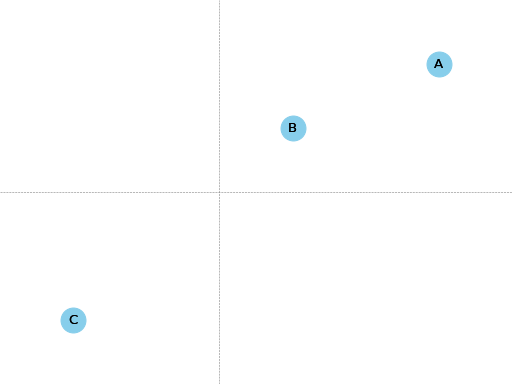
A is much closer to B.

Here’s the mental leap. Embeddings are similar to points on a map.
Each number in the embedding array is a dimension, similar to the
X-Coordinates and Y-Coordinates from earlier. When an embedding
model sends you back an array of 1000 numbers, it’s telling you the
point where that text semantically lives in its 1000-dimension space,
relative to all other texts. When we compare the distance between two
embeddings in this 1000-dimension space, what we’re really doing is
figuring out how semantically close or far apart those two texts are
from each other.

The concept of positioning items in a multi-dimensional
space like this, where related items are clustered near each other,
goes by the wonderful name of latent space.

The most famous example of the weird utility of this technology comes from
the Word2vec paper, the foundational research that kickstarted interest
in embeddings 11 years ago. In the paper they shared this anecdote:

embedding("king") - embedding("man") + embedding("woman") ≈ embedding("queen")

Starting with the embedding for king, subtract the embedding for man,
then add the embedding for woman. When you look around this vicinity of the
latent space, you find the embedding for queen nearby. In other words,
embeddings can represent semantic relationships in ways that feel intuitive
to us humans. If you asked a human “what’s the female equivalent
of a king?” that human would probably answer “queen”, the same answer we get from embeddings. For more explanation of the underlying theories, see Distributional semantics.

The 2D map analogy was a nice stepping stone for building intuition but now we need
to cast it aside, because embeddings operate in hundreds or thousands
of dimensions. It’s impossible for us lowly 3-dimensional creatures to
visualize what “distance” looks like in 1000 dimensions. Also, we don’t know
what each dimension represents, hence the section heading “Very weird
multi-dimensional space”.⁵ One dimension might represent something
close to color. The king - man + woman ≈ queen anecdote suggests that these
models contain a dimension with some notion of gender. And so on.
Well Dude, we just don’t know.

The mechanics of converting text into very weird multi-dimensional space are
complex, as you might imagine. They are teaching machines to LEARN, after all.
The Illustrated Word2vec is a good way to start your journey down that
rabbithole.

⁵ I borrowed this phrase from Embeddings: What they are and why they
matter.

Comparing embeddings§

After you’ve generated your embeddings, you’ll need some kind of “database”
to keep track of what text each embedding is associated to. In the experiment
discussed later, I got by with just a local JSON file:

{
    "authors": {
        "embedding": […]
    },
    "changes/0.1": {
        "embedding": […]
    },
    …
}

authors is the name of a page. embedding is the embedding for that page.

Comparing embeddings involves a lot of linear algebra.
I learned the basics from Linear Algebra for Machine Learning and Data Science.
The big math and ML libraries like NumPy and scikit-learn can do the
heavy lifting for you (i.e. very little math code on your end).

Related pages§

Some docs sites have a recommendation system that makes you aware of other
relevant docs. The system looks at whatever page you’re currently on, finds
other pages related to this one, and then recommends other pages to visit.
Embeddings provide a new way to support this feature, probably at a fraction
of the cost of previous methods. Here’s how it works:

1. Generate an embedding for each page on your docs site.

2. For each page, compare its embedding against all other page embeddings.
   If the two embeddings are mathematically similar, then the contents
   on the two pages are probably related to each other.

This can be done as a batch operation. A page’s embedding only needs to
change when the page’s content changes.

I ran this experiment on the Sphinx docs. The results were pretty good.
Implementation and
Results have the details.

See Related content using embeddings for another example of this approach.

Let a thousand embeddings bloom?§

As docs site owners, I wonder if we should start freely providing embeddings for our
content to anyone who wants them, via REST APIs or well-known URIs.
Who knows what kinds of cool stuff our communities can build with this extra type
of data about our docs?

Implementation§

I created a Sphinx extension to generate an embedding for each doc. Sphinx automatically invokes
this extension as it builds the docs.

import json
import os


import voyageai


VOYAGE_API_KEY = os.getenv('VOYAGE_API_KEY')
voyage = voyageai.Client(api_key=VOYAGE_API_KEY)


def on_build_finished(app, exception):
    with open(srcpath, 'w') as f:
        json.dump(data, f, indent=4)


def embed_with_voyage(text):
    try:
        embedding = voyage.embed([text], model='voyage-3', input_type='document').embeddings[0]
        return embedding
    except Exception as e:
        return None


def on_doctree_resolved(app, doctree, docname):
    text = doctree.astext()
    embedding = embed_with_voyage(text)  # Generate an embedding for each document!
    data[docname] = {
        'embedding': embedding
    }


# Use some globals because this is just an experiment and you can't stop me
def init_globals(srcdir):
    global filename
    global srcpath
    global data
    filename = 'embeddings.json'
    srcpath = f'{srcdir}/{filename}'
    data = {}


def setup(app):
    init_globals(app.srcdir)
    # https://www.sphinx-doc.org/en/master/extdev/appapi.html#sphinx-core-events
    app.connect('doctree-resolved', on_doctree_resolved)  # This event fires on every doc that's processed
    app.connect('build-finished', on_build_finished)
    return {
        'version': '0.0.1',
        'parallel_read_safe': True,
        'parallel_write_safe': True,
    }

When the build finishes, the embeddings data is stored in embeddings.json like this:

{
    "authors": {
        "embedding": […]
    },
    "changes/0.1": {
        "embedding": […]
    },
    …
}

authors and changes/0.1 are docs. embedding contains the
embedding for that doc.

The last step is to find the closest neighbor for each doc. I.e. to
find the other page that is considered relevant to the page you’re currently on.
As mentioned earlier, Linear Algebra for Machine Learning and Data Science
was the class that taught me the basics.

import json


import numpy as np
from sklearn.metrics.pairwise import cosine_similarity


def find_docname(data, target):
    for docname in data:
        if data[docname]['embedding'] == target:
            return docname
    return None


# Adapted from the Voyage AI docs
# https://web.archive.org/web/20240923001107/https://docs.voyageai.com/docs/quickstart-tutorial
def k_nearest_neighbors(target, embeddings, k=5):
    # Convert to numpy array
    target = np.array(target)
    embeddings = np.array(embeddings)
    # Reshape the query vector embedding to a matrix of shape (1, n) to make it
    # compatible with cosine_similarity
    target = target.reshape(1, -1)
    # Calculate the similarity for each item in data
    cosine_sim = cosine_similarity(target, embeddings)
    # Sort the data by similarity in descending order and take the top k items
    sorted_indices = np.argsort(cosine_sim[0])[::-1]
    # Take the top k related embeddings
    top_k_related_embeddings = embeddings[sorted_indices[:k]]
    top_k_related_embeddings = [
        list(row[:]) for row in top_k_related_embeddings
    ]  # convert to list
    return top_k_related_embeddings


with open('doc/embeddings.json', 'r') as f:
    data = json.load(f)
embeddings = [data[docname]['embedding'] for docname in data]
print('.. csv-table::')
print('   :header: "Target", "Neighbor"')
print()
for target in embeddings:
    dot_products = np.dot(embeddings, target)
    neighbors = k_nearest_neighbors(target, embeddings, k=3)
    # ignore neighbors[0] because that is always the target itself
    nearest_neighbor = neighbors[1]
    target_docname = find_docname(data, target)
    target_cell = f'`{target_docname} <https://www.sphinx-doc.org/en/master/{target_docname}.html>`_'
    neighbor_docname = find_docname(data, nearest_neighbor)
    neighbor_cell = f'`{neighbor_docname} <https://www.sphinx-doc.org/en/master/{neighbor_docname}.html>`_'
    print(f'   "{target_cell}", "{neighbor_cell}"')

As you may have noticed, I did not actually implement the recommendation
UI in this experiment. My main goal was to get basic data on whether
the embeddings approach generates decent recommendations or not.

Results§

How to interpret the data: Target would be the page that you’re
currently on. Neighbor would be the recommended page.