Geometrically understanding calculus of inverse functions (2023)

Given a function such as (tan x), could you write (frac{d}{dx} arctan x) and (int arctan x ; dx), just from (tan x), (frac{d}{dx} tan x) and (int tan x ; dx)? With some caveats, the inverse function theorem answers the former while the Legendre transformation answers the later. We’ll approach this with as much geometric intuition as possible, avoiding the dry application of formulas.

Derivatives of inverse functions and the inverse function theorem

Instead of approaching the inverse function theorem through formulas, we’ll explore it geometrically—it’s much more intuitive and enjoyable!

But first, to refresh our memory, let’s revisit the formal statement of the inverse function theorem, which relates the derivative of (f(x)) and its inverse (f^{-1}(x)).

Given a continuously differentiable function (f: mathbb{R} to mathbb{R}) with (f'(a) neq 0) at some point, the inverse function theorem states that there is some interval (I) with (a in I) such that there exists a continuously differentiable inverse (f^{-1}) defined on (f(I)) such that for all (x in I)

[frac{df^{-1}}{dx}(x) = frac{1}{f'(f^{-1}(x))}.]

A simple example of the theorem in action is finding the derivative of (ln x), which evaluates to (1/e^{ln x} = 1/x). The standard high school approach to deduce the above in high school is to differentiate both sides of (f^{-1}(f(x)) = x).

This formal approach is quite dry and things get a lot more interesting when we think geometrically.

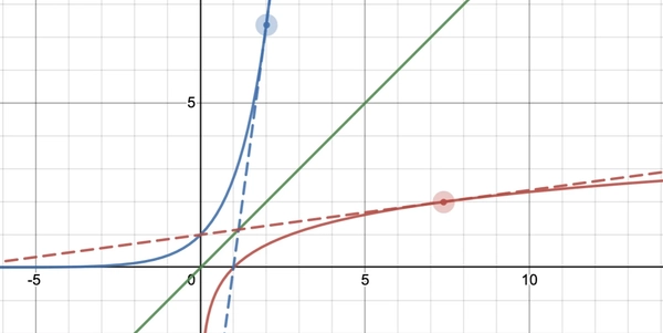
Geometrically, given some function (f(x) = y) the inverse is just taking the plot of the function and reflecting it about the diagonal line (y=x). As such all tangent lines are also reflected along the diagonal line and hence the slope is inversed. Below we have the graph of (e^x) (the blue line) and the graph of (ln x) (the red line). And you can see how the tangent line of (e^x) at ((2,e^2)) is reflected along (y=x) to give the tangent line of (ln x) at ((e^2, 2)).

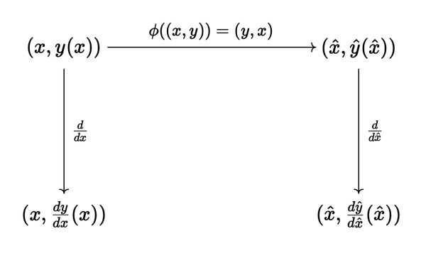
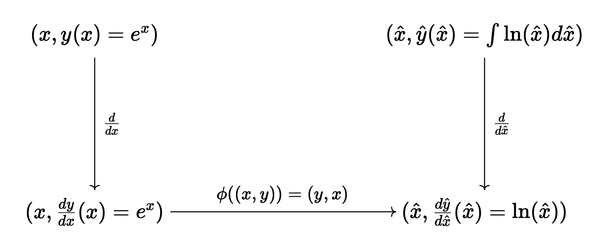
Another way of looking at it would be to subjugate (S={(x, f(x)) , vert , x in I}), the plot of (f(x)), with a graph transformation (phi:(x,y) to (hat{x}, hat{y}) = (y,x)) and express (phi(S)) as a plot ((hat{x}, hat{y}(hat{x}))). This way (hat{y}) would be in effect the inverse of (y). We then wish to understand how (phi) acts on (frac{dy}{dx}) to give (frac{dhat{y}}{dhat{x}}).

You can express this with the following graph

and the equalities

[begin{align*}
hat x(x) &= y(x), \
hat y(hat x(x)) &= x \
&= y^{-1}(hat x(x)).
end{align*}]

We could then directly calculate

[begin{align*}
frac{dhat{y}}{dhat{x}}(hat x(x)) &= frac{dhat{y}}{dx}(x) / frac{dhat{x}}{dx}(x) & text{(Chain rule)} \
&= 1 / frac{dy}{dx}(x).
end{align*}]

This recovers the inverse function theorem.

This method generalises to other maps (phi: mathbb{R}^2 to mathbb{R}^2) (e.g. (phi:(r, theta) to (r cos theta, r sin theta))) . These ideas are explored much more deeply in Hydon’s book on Symmetry Methods for Differential Equations.

By calculating (frac{d}{dx} tan x = sec^2 x), we now know that (frac{d}{dx} arctan x = frac{1}{text{sec}^2(arctan x)} = frac{1}{1+x^2}). So what about (int arctan x , dx)?

Integrals of inverse functions and the Legendre transformation

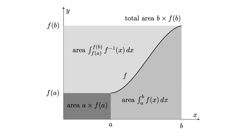
Geometrically, we could show that with (f) strictly monotone, we have

[int_{f(a)}^{f(b)} f^{-1}(y) , dy + int^{b}_a f(x) , dx = bf(b)-af(a)]

This is a result by Laisant in 1905. Here’s a proof-without-words.

<!– By Jonathan Steinbuch – Own work,
CC BY-SA 3.0, Link –>

You can use this to recover the explicit formula of the integral of (f^{-1}), which is left as an exercise! Instead we will use the graph reflection approach used earlier for the inverse function theroem.

Suppose we’re interested in finding (int arctan x , dx). Notationally, it is the easiest to let (y = int tan x , dx) up to some constant such that (frac{dy}{dx} = tan x) is the function we want to invert. Let (S) be the plot of (frac{dy}{dx}), i.e. ({(x, frac{dy}{dx}) vert , x in I}) for some appropiate interval (I). Applying the map (phi: (x,y) to (hat{x}, hat{y}) = (y,x)), we assume the existence of some (hat{y}) such that its derivative is the plot of (phi(S)). Now (hat{y} = int arctan hat{x} , dhat{x}) which is what we seek.

Consider

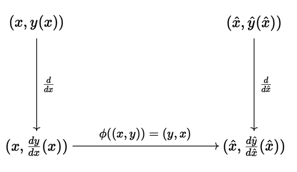
with the equalities

[begin{align*}
hat x(x) &= frac{dy}{dx}(x), \
frac{dhat y}{dhat x}(hat x(x)) &= x. \
end{align*}]

Now consider

[begin{align*}
&;hat{y}(hat{x}) \
&= intfrac{dhat y}{dhat x}(hat{x}) dhat{x} \
&= hat{x} frac{dhat y}{dhat x}(hat{x}) – int hat{x}frac{d^2hat y}{dhat x^2}(hat{x}) dhat{x} & (text{by parts}) \
&= hat{x} frac{dhat y}{dhat x}(hat{x}) – int hat{x}(x)frac{d^2hat y}{dhat x^2}(hat{x}(x)) frac{dhat x}{dx}(x) dx &\
&= hat{x} frac{dhat y}{dhat x}(hat{x}) – int hat{x}(x)bigg[frac{d}{dx}bigg(frac{dhat y}{dhat x}(hat{x}(x))bigg)(x)bigg] dx & (text{chain rule})\
&= hat{x} frac{dhat y}{dhat x}(hat{x}) – int hat{x}(x) dx & bigg(frac{dhat y}{dhat x}(hat{x}(x)) = xbigg) \
&= hat{x} frac{dhat y}{dhat x}(hat{x}) – int frac{dy}{dx}(x) dx & (text{by def of } hat{x})\
&= hat{x} frac{dhat y}{dhat x}(hat{x}) – y(x) + C \
&= hat{x} frac{dhat y}{dhat x}(hat{x}) – ybigg(frac{dhat{y}}{dhat x}(hat{x})bigg) + C. & (text{by def of } hat{x})
end{align*}]

Let’s try to compute a simple example, the integral of (ln x). Consider

Repeating what we’ve done above, we have

[begin{align*}
hat{y} &= int ln hat{x} , dhat{x} \
&= hat{x} times ln(hat{x}) – int hat{x} times frac{d}{dhat x}(ln hat{x}) dhat{x}\
&= hat{x} times ln(hat{x}) – int e^x times frac{d}{dhat x}(ln hat x) times frac{d}{dx} (hat x) dx \
&= hat{x} times ln(hat{x}) – int e^x times frac{d}{dx} big(ln(e^x)big) dx \
&= hat{x} times ln(hat{x}) – int e^x dx \
&= hat{x} times ln(hat{x}) – e^x + C \
&= hat{x} times ln(hat{x}) – e^{ln (hat{x})} + C \
&= hat{x} times ln(hat{x}) – hat{x} + C.
end{align*}]

Finally, just by using the formula (hat{y} = hat{x} timesfrac{dhat y}{dhat x}(hat{x}) – y(hat{y}'(hat{x})) + C), if we let (y = – ln vert cos(x) vert), then we have (y’ = tan(x)) and (hat{y}’ = arctan(x)) so

[begin{align*}
int arctan hat{x} &= hat{x} arctan hat{x} – ln vert cos(arctan(hat{x}))vert + C\
&= hat{x} arctan hat{x} – frac{1}{2} ln big( frac{1}{1+hat{x}^2}big) + C
end{align*}]

as expected.

The map (y(x) to hat{y}(hat{x}) := hat{x}frac{dhat y}{dhat x}(hat{x}) – y(frac{dhat y}{dhat x}(hat{x}))) is called the Legendre transformation, which has wide applications in areas of physics. But mathematically, one could think of it as an analogue to the inverse function theorem: It tells you how the inverse map acts on integrals.

Summary

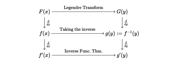
with the following relations

[begin{align*}
text{IFT:} quad & g'(y) = frac{1}{f'(g(y))} \
text{Legendre:} quad & G(y) = ytimes g(y) – F(g(y)) + C
end{align*}]

For more ways to understand the ideas covered in this post you can look at the article I’ve written for the Oxford Invariants journal, as well as the wiki page on the integral of inverse functions.

<!– Next post

Previous post

All posts in “maths”

–>